从装有\(N\)个球,其中\(K\)个白球的袋子中不放回的抽取n个球,n个球中白球个数的分布即为超几何分布,wiki百科上有关于超几何分布的详尽介绍,但是没有两个重要数字特征,期望和方差的推导,本文将用两种方法对这两个数字特征进行数学推导。 Let \(X\) denote the number of white balls selected when \(n\) balls are chosen at random from an urn containing \(N\) balls \(K\) of which are white. The distribution of \(X\) is Hypergeometric Distribution. You can find detail description at Wikipedia, but the derivation of Expectation and Variance is omitted. I’ll show the derivation here from two different aspects.
First, Just Do It! Obviously, $$\begin{align} P\{X=i\} &= \frac{{K \choose i}{N-K \choose n-i}}{{N \choose n}} \\ N &\in \{0, 1, 2, \dots\} \\ K &\in \{0, 1, 2, \dots, N\} \\ n &\in \{0, 1, 2, \dots, N\} \\ i &\in \{max(0, n+K-N), \dots, min(n, K)\}\\ \\ E[X] &= \sum iP\{X=i\} =\frac{i{K \choose i}{N-K \choose n-i}}{{N \choose n}} \\ &= K\sum \frac{{K-1 \choose i-1}{N-K \choose n-i}}{{N \choose n}} \end{align}$$ We find the latter part in sum is very similar to the sum of the probability of a variable obeying hypergeometric distribution(which will equal to 1). Thus we do some transformations and get, $$\begin{align} E[X] &= K\sum \frac{{K-1 \choose i-1}{(N-1)-(K-1) \choose (n-1)-(i-1)}}{\frac{N}{n}{N-1 \choose n-1}} \\ &= \frac{kn}{N} \sum \frac{{K-1 \choose i-1}{(N-1)-(K-1) \choose (n-1)-(i-1)}}{{N-1 \choose n-1}} \\ &= \frac{kn}{N} \\ \end{align}$$ We can do it recursively and get, $$\begin{align} E[X(X-1)] &= \frac{K(K-1)n(n-1)}{N(N-1)} \sum \frac{{K-2 \choose i-2}{(N-2)-(K-2) \choose (n-2)-(i-2)}}{{N-2 \choose n-2}} \\ &= \frac{K(K-1)n(n-1)}{N(N-1)} \\ Var(X) &= E[X^2] – E^2[X] = E[X(X-1)] + E[X] – E^2[X]\\ &= \frac{Kn(N-K)(N-n)}{N^2(N-1)} \end{align}$$
It’s very time-consuming. Though hardcore, it works. Next I want to introduce a smarter way.
Second, Divide and Conquer!
Let \(X_i\) to be the \(ith\) ball in the N balls and \(X_i = 1\) if it’s white, it’s easy to see that \(P(X_i = 1) = \frac{K}{N}\) which is independent from the position \(i\) and whether the balls was removed after chosen. So we get, $$\begin{align} E[X_i] &= \frac{K}{N}\\ Var(X_i) &= \frac{K(N-K)}{N^2} \end{align}$$ And we can easily get the expectation, $$ E[X] = \sum_{n}E[X_i] = \frac{Kn}{N} $$ Though all the \(X_i\) obeys the same distribution, they are not independent. To calculate the variance, we have to compute their covariance first. $$\begin{align} Cov(X_i, X_j) &= E[X_i X_j] – E[X_i]E[X_j] \\ &= P\{X_i = 1, X_j = 1\} – \frac{K^2}{N^2}\\ &= P\{X_i = 1 | X_j = 1\}P\{X_j = 1\} – \frac{K^2}{N^2}\\ &= \frac{K-1}{N-1} \frac{K}{N} – \frac{K^2}{N^2}\\ &= -\frac{K(N-K)}{N^2(N-1)}\\ Var(X) &= \sum Var(X_i) + \sum_{i\neq j}Cov(X_i, X_j) \\ &= n\frac{K(N-K)}{N^2} – n(n-1)\frac{K(N-K)}{N^2(N-1)} \\ &= \frac{Kn(N-K)(N-n)}{N^2(N-1)} \end{align}$$
A Little More 🙂
Since all \(X_i\) obeys the same distribution, and is independent from the position \(i\) and whether the balls was removed after chosen, we can also conclude that “Draw Lots” is a fair game. Regardless the order you draw the lot, you get the equal probability.
《随机过程-第二版》(英文电子版) Sheldon M. Ross 答案整理,此书作为随机过程经典教材没有习题讲解,所以将自己的学习过程记录下来,部分习题解答参考了网络,由于来源很多,出处很多也不明确,无法一一注明,在此一并表示感谢!希望对大家有帮助,水平有限,不保证正确率,欢迎批评指正,转载请注明出处。 Solutions to Stochastic Processes Sheldon M. Ross Second Edition(pdf) Since there is no official solution manual for this book, I handcrafted the solutions by myself. Some solutions were referred from web, most copyright of which are implicit, can’t be listed clearly. Many thanks to those authors! Hope these solutions be helpful, but No Correctness or Accuracy Guaranteed. Comments are welcomed. Excerpts and links may be used, provided that full and clear credit is given.
1.1 Let \(N\) denote a nonnegative integer-valued random variable. Show that $$E[N]= \sum_{k=1}^{\infty} P\{N\geq k\} = \sum_{k=0}^{\infty} P\{N > k\}.$$
In general show that if \(X\) is nonnegative with distribution \(F\), then $$E[X] = \int_{0}^{\infty}\overline{F}(x)dx $$
and $$E[X^n] = \int_{0}^{\infty}nx^{n-1}\overline{F}(x)dx. $$
1.2 If \(X\) is a continuous random variable having distribution \(F\) show that. (a) \( F(X)\) is uniformly distributed over(0, 1), (b) if \(U\) is a uniform (0, 1) random variable, then \(F^{-1}(U)\) has distribution \(F\), where \(F^{-1}(x)\) is that value of \(y\) such that \(F(y)=x\)
(a) Let \(Z = F(X)\), $$ \begin{align} F_Z(x) &= P\{Z \leq x\} = P\{F_X(X) \leq x\} \\ &= P \{X \leq F_X^{-1}(x)\} \quad (F(x) \text{ is invertible and non-decreasing})\\ &= F_X(F_X^{-1}(x))\\ &= x \end{align}$$
(b) Let \(Z = F^{-1}(U)\), $$ \begin{align} F_Z(x) &= P\{Z \leq x\} = P\{F^{-1}(U) \leq x\} \\ &= P \{U \leq F(x)\} \quad (F(x) \text{ is invertible and non-decreasing})\\ &= F_U(F(x))\\ &= F(x) \end{align}$$
1.3 Let \(X_n\) denote a binomial random variable with parameters \((n, p_n), n \geq 1\) If \(np_n \rightarrow \lambda\) as \(n \rightarrow \infty\), show that $$P\{X^n = i\} \rightarrow e^{-\lambda}\lambda^i/i! \quad as\enspace n \rightarrow \infty.$$
1.7 Let \(X\) denote the number of white balls selected when \(k\) balls are chosen at random from an urn containing \(n\) white and \(m\) black balls. Compute \(E[X]\) and \(Var(X)\) .
Obviously, \(X \sim H(m+n, n, k) \) Thus, $$\begin{align} E(X) &= \frac{kn}{m+n}\\ Var(X) &= \frac{kmn}{(m+n)^2} (\frac{n+m-k}{n-k}) \end{align}$$ More about Hypergeometric Distribution from wikipedia.org, I’ve also written down the derivation in this post.
1.8 Let \(X_1\) and \(X_2\) be independent Poisson random variables with means \(\lambda_1\) and \(\lambda_2\). (a) Find the distribution of \(X_1 + X_2\) (b) Compute the conditional distribution of \(X_1\) given that \(X_1 + X_2 = n\)
1.9 A round-robin tournament of \(n\) contestants is one in which each of the \({n \choose 2}\) pairs of contestants plays each other exactly once, with the outcome of any play being that one of the contestants wins and the other loses. Suppose the players are initially numbered \(1, 2, \dots, n\). The permutation \(i_1, \dots, i_n\) is called a Hamiltonian permutation if \(i_1\) beats \(i_2\), \(i_2\) beats \(i_3, \dots\) and \(i_{n-1}\) beats \(i_n\). Show that there is an outcome of the round-robin for which the number of Hamiltonian is at least \(n!/2^{n-1}\). (Hint. Use the probabilistic method.)
\(Proof:\) Suppose \(X\) be the permutation number of a n contestants Hamiltonian permutation which start at particular contestant, the expectation is \(E_n\), the total number’s expectation will be \(nE_n\). Also we suppose each game equally likely to be won by either contestant, independently. Thus, $$\begin{align} E_n &= \sum {n-1 \choose k}(\frac{1}{2})^k (\frac{1}{2})^{n-1-k} k E_{n-1} \\ &= \frac{(n-1)E_{n-1}}{2} \sum {n-2 \choose k-1} (\frac{1}{2})^{k-1} (\frac{1}{2})^{n-1-k} \\ &= \frac{(n-1)E_{n-1}}{2} \\ &= \frac{(n-1)!}{2^n}E_1 \\ \end{align}$$ Obviously, \(E_1 = 1, nE_n = n!/2^{n-1} \). Since at least one of the possible values of a random variable must be at least as large as its mean, proven.
1.11 If \(X\) is a nonnegative integer-valued random variable then the function \(P(z)\), defined for \(|z| \leq 1\) by $$P(z) = E[z^X] = \sum_{j=0}^{\infty} z^j P\{X=j\}$$ is called the probability generating function of \(X\) (a) Show that $$\frac{d^k}{dz^k}P(z)_{|z=0} = k!P\{X=k\}.$$ (b) With 0 being considered even, show that $$P\{X\ is\ even\} = \frac{P(-1) + P(1)}{2}$$ (c) If \(X\) is binomial with parameters \(n\) and \(p\), show that $$ P\{X\ is\ even\} = \frac{1 + (1-2p)^n}{2} $$ (d) If \(X\) is Poisson with mean \(\lambda\), show that $$ P\{X\ is\ even\} = \frac{1 + e^{-2\lambda}}{2} $$ (e) If \(X\) is geometric with parameter p, show that, $$ P\{X\ is\ even\} = \frac{1-p}{2-p} $$ (f) If \(X\) is a negative binomial random variable with parameters \(r\) and \(p\), show that $$ P\{X\ is\ even\} = \frac{1}{2} [1 + (-1)^r (\frac{p}{2-p})^r] $$
1.12 If \(P\{0 \leq X \leq a\} = 1\), show that $$ Var(X) \leq a^2 / 4. $$
\(Proof:\) $$\begin{align} Var(X) &= E[X^2] – E^2[X] = \int_0^a x^2 dF(x) – [\int_0^a x dF(x)]^2 \\ &= x^2 F(x)|_0^a – 2\int_0^a xF(x) dx – [xF(x)|_0^a – \int_0^a F(x) dx ]^2 \\ &= -[\int_0^a F(x) dx ]^2 – 2\int_0^a (x-a)F(x) dx \\ &\leq -[\int_0^a F(x) dx ]^2 – \frac{2}{a}\int_0^a (x-a)dx\int_0^a F(x) dx \quad \text{(Chebyshev’s sum inequality)}\\ &= -t^2 + at \quad (t = \int_0^a F(x) dx) \\ \end{align}$$ When \(t = a/2 \) we get the max value, which is \(a^2 / 4\), proven.
1.13 Consider the following method of shuffling a deck of \(n\) playing cards, numbered 1 through \(n\). Take the top card from the deck and then replace it so that it is equally likely to be put under exactly \(k\) cards, for \(k = 0, 1, \dots , n-1\). Continue doing this operation until the card that was initially on the bottom of the deck is now on top. Then do it one more time and stop. (a) Suppose that at some point there are \(k\) cards beneath the one that was originally on the bottom of the deck. Given this set of \(k\) cards explain why each of the possible \(k!\) orderings is equally likely to be the ordering of last \(k\) cards. (b) Conclude that the final ordering of the deck is equally likely to be any of the \(N!\) possible orderings. (c) Find the expected number of times the shuffling operation is performed.
(a) Consider there are k numbered positions that can be inserted at the beginning, every card has the same probability to be inserted into any of the k position. That’s to say every ordering has the same probability. (b) Let k = n. (c) Let \(X_i\) denote the number of operations performed to add the ith card to the \(i-1\) cards beneath the “bottom card”. Obviously, \(X_i \sim G(i/n)\), and total number is \(X\), $$ E[X] = E[\sum_{i=1}^{n-1} X_i] + 1 = \sum_{i=1}^{n-1} E[X_i] + 1 = \sum_{i=1}^{n} \frac{n}{i} $$
(c)Wrong attempt: Let \(X_i\) denote number of cards beneath the “bottom card” in the \(ith\) perform, then we have $$\begin{align} E[X_i] &= E[E[X_i| X_{i-1} = k]] \\ &= E[(k+1)\frac{k+1}{n} + k(1-\frac{k+1}{n})] \\ &= \frac{n+1}{n}E_{i-1} + \frac{1}{n}\\ &= (\frac{n+1}{n})^i – 1 \quad (E[X_1] = 1/n) \\ \end{align}$$ Let \(E[X_i] = n – 1\), solved \(i + 1 = \ln {(n+1)}/(\ln{(n+1)} – \ln{n})\), which is the expected times.
1.15 Let \(F\) be a continuous distribution function and let \(U\) be a uniform (0, 1) random variable. (a) If \(X= F^{-1}(U)\), show that \(X\) has distribution function \(F\). (b) Show that \(-\ln{U}\) is an exponential random variable with mean 1.
(a) See Problem 1.2(b). (b) Since \(F^{-1}(U) = -\ln{U}, F(x) = e^{-x}\), thus, \( (-\ln{U}) \sim Exponential(1) \) \( E[-\ln{U}] = 1 \)
1.16 Let \(f(x)\) and \(g(x)\) be probability density functions, and suppose that for some constant \(c\), \(f(x) \leq cg(x)\) for all x. Suppose we can generate random variables having density function \(g\), and consider the following algorithm. Step 1: Generate \(Y\), a random variable having density function \(g\). Step 2: Generate \(U\), a uniform (0, 1) random variable. Step 3: If \(U \leq \frac{f(Y)}{cg(Y)}\) set \(X = Y\). Otherwise, go back to Step 1. Assuming that successively generated random variables are independent, show that: (a) \(X\) has density function \(f\) (b) the number of iterations of the algorithm needed to generate \(X\) is a geometric random variable with mean \(c\)
(b) Suppose the \(p\) is probability to generate \(X\), then, $$\begin{align} p &= P\{U \leq \frac{f(Y)}{cg(Y)}\} \\ &= \int_{-\infty}^{\infty} \frac{f(y)}{cg(y)} g(y)dy \\ &= \frac{1}{c} \int_{-\infty}{\infty} f(y)dy \\ &= \frac{1}{c} \end{align}$$ Obviously, the number of iterations needed is \(G(\frac{1}{c})\), whose mean is \(c\).
(a) $$\begin{align} f_x(y) &= P\{Y = y | U \leq \frac{f(Y)}{cg(Y)}\} \\ &= cP\{Y = y, U \leq \frac{f(y)}{cg(y)}\} \\ &= cg(y)P\{U \leq \frac{f(y)}{cg(y)}\} \\ &= cg(y) \frac{f(y)}{cg(y)} \\ &= f(y) \end{align}$$
This is called Acceptance-Rejection Method, refer this paper for detail.
1.17 Hint: \(P\{X_n \text{is the ith smallest}\} = \int {n-1 \choose i-1}F(x)^{i-1}\overline F(x)^{n-i}dF(x)\), do partial integration repeatedly, we get the probability is \(1/n\). This is called Order Statistic, more detail at Wikipedia.
1.18 A coin, which lands on heads with probability \(p\), is continually flipped. Compute the expected number of flips that are made until a string of \(r\) heads in a row is obtained.
Let \(X\) denote the number of flips that are made until a string of \(r\) heads in a row is obtained. Let \(Y\) denote the number of flips until the first occurrence of tails. Then \(P\{Y=i\}=p^{i-1}(1-p)\). When \(i \leq r\), we start over again, \(E(X|Y=i) = i + E(X)\), and if \(i > r, E[X|Y=i] = r\). Thus, $$\begin{align} E[X] &= \sum_{i=1}^{\infty} E[X|Y=i]P\{Y=i\} \\ &= (1-p) \sum_{i=1}^{r}p^{i-1}(i + E[X]) + (1-p)\sum_{i=r+1}^{\infty} p^{i-1}r \\ &= (1-p) \sum_{i=1}^{r}ip^{i-1} + E[X](1-p^r) + rp^r \\ \end{align}$$ Let \(S = \sum_{i=1}^{r}ip^{i-1} \), then \((1-p)S = \sum_{i=1}^r p^{i-1} – rp^r = \frac{1-p^r}{1-p} – rp^r \) . Hence, $$\begin{align} E[X] &= \frac{1-p^r}{1-p} – rp^r + E[X](1-p^r) + rp^r \\ &= \frac{1-p^r}{1-p} + E[X](1-p^r) \\ &= \frac{1-p^r}{p^r(1-p)} \end{align}$$
1.19 An urn contains \(a\) white and \(b\) black balls. After a ball is drawn, it is returned to the urn if it is white; but if it is black, it is replaced by a white ball from another urn. Let \(M_n\) denote the expected number of white balls in the urn after the foregoing operation has been repeated \(n\) times. (a) Derive the recursive equation $$M_{n+1} = (1 – \frac{1}{a+b})M_n + 1.$$ (b) Use part (a) to prove that $$M_n = a + b – b(1 – \frac{1}{a+b})^n$$ (c) What is the probability that the (n+1)st ball drawn is white?
(a) Let \(X_n\) denote the number of white balls after \(n\) operations, then, $$\begin{align} M_{n+1} &= E[E[X_{n+1}|X_n=k]] \\ &= E[k\frac{k}{a+b} + (k+1)(1 – \frac{k}{a+b})] \\ &= (1 – \frac{1}{a+b})E[k] + 1 \\ &= (1 – \frac{1}{a+b})M_n + 1 \end{align}$$ (b) $$\begin{align} M_n – (a+b) &= (1 – \frac{1}{a+b})(M_{n-1} – (a+b)) \\ &= (M_0 – a – b)(1 – \frac{1}{a+b})^n \\ M_n &= a + b – b (1 – \frac{1}{a+b})^n \\ \end{align}$$ (c) Let \(I_n = 1\) denote the nth ball drawn is white, \(I_n = 0\) when black. then, $$\begin{align} P\{(n+1)st \text{ ball is white}\} &= E[I_{n+1}] = E[E[I_{n+1} | X_n = k]] \\ &= \frac{M_n}{a+b} \end{align}$$
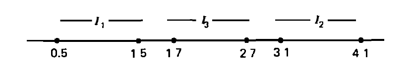
1.20 A Continuous Random Packing Problem Consider the interval \((0, x)\) and suppose that we pack in this interval random unit intervals–whose left-hand points are all uniformly distributed over \((0, x-1)\) — as follows. Let the first such random interval be \(I_1\). If \(I_1, \dots , I_k\) have already been packed in the interval, then the next random unit interval will be packed if it dose not intersect any of the intervals \(I_1, \dots , I_k\), and the interval will be denoted by \(I_{k+1}\). If it dose intersect any of the intervals \(I_1, \dots , I_k\), we disregard it and look at the next random interval. The procedure is continued until there is no more room for additional unit intervals (that is, all the gaps between packed intervals are smaller than 1). Let \(N(x)\) denote the number of unit intervals packed in \([0, x]\) by this method. For instance, if \(x=5\) and the successive random intervals are \((0.5, 1.5),\ (3.1, 4.1),\ (4, 5),\ (1.7, 2.7)\), then \(N(5) = 3\) with packing as follows
Let \(M(x) = E[N(x)]\), Show that \(M\) satisfies $$\begin{align} M(x) &= 0 \quad \quad x < 1,\\ M(x) &= \frac{2}{x-1}\int_0^{x-1} M(y)dy + 1, \quad x>1 \end{align}$$
Let \(Y\) denote the left-hand point of the first interval, \(Y \sim U(0, x-1)\), and the first interval divide the whole into two parts with length y and x – y -1, hence $$\begin{align} M(x) &= E[N(x)] = E[E[N(x) | Y]] \\ &= E[N(y) + N(x-y-1) + 1] \\ &= \int_0^{x-1} (\frac{1}{x-1})[M(y) + M(x-y-1) + 1] dy \\ &= \frac{2}{x-1}\int_0^{x-1} M(y)dy + 1, \quad x>1 \end{align}$$
1.23 Consider a particle that moves along the set of integers in the following manner. If it is presently at \(i\) then it next moves to \(i + 1\) with probability \(p\) and to \(i-1\) with probability \(1-p\). Starting at 0, let \(\alpha\) denote the probability that it ever reaches 1. (a) Argue that $$\alpha = p + (1-p) \alpha^2$$ (b) Show that $$ \alpha = \left\{ \begin{array}{ll} 1 \quad p \geq 1/2 \\ p/(1-p) \quad p < 1/2 \\ \end{array} \right. $$ (c) Find the probability that the particle ever reaches \(n, n > 0 \) (d) Suppose that \(p<1/2\) and also that the particle eventually reaches \(n, n > 0\). If the particle is presently at \(i, i<n\), and \(n\) has not yet been reached, show that the particle will next move to \(i+1\) with probability \(1-p\) and to \(i-1\) with probability \(p\). That is, show that $$P\{\text{next at } i + 1 | \text{at } i \text{ and will reach n}\} = 1-p$$ (Note that the roles of \(p\) and \(1-p\) are interchanged when it is given that \(n\) is eventually reached)
(a) Obviously (b) Solve the equation in (a), get \(\alpha=1\) or \(\alpha= p/(1-p)\). Since \(\alpha \leq 1\), $$ \alpha = \left\{ \begin{array}{ll} 1 \quad p \geq 1/2 \\ p/(1-p) \quad p < 1/2 \\ \end{array} \right. $$ (c) $$\alpha^n = \frac{p^n}{(1-p)^n}$$ (d) $$\begin{align} &P\{\text{next at } i + 1 | \text{at } i \text{ and will reach n}\} \\ &= \frac{P\{\text{at } i \text{ and will reach n} | \text{next at } i + 1 \} \cdot p}{P\{\text{at } i \text{ and will reach n}\} } \\ &= \frac{p\cdot p^{n-i-1}}{(1-p)^{n-i-1}} / \frac{p^{n-i}}{(1-p)^{n-i}} \\ &= 1- p \end{align}$$
1.24 In Problem 1.23, let \(E[T]\) denote the expected time until the particle reaches 1. (a) Show that $$E[T] = \left\{ \begin{array}{ll} 1/(2p – 1) \quad p > 1/2 \\ \infty \quad p \leq 1/2 \\ \end{array} \right.$$ (b) Show that, for \(p > 1/2\), $$Var(T) = \frac{4p(1-p)}{(2p-1)^3}$$ (c) Find the expected time until the particle reaches \(n, n > 0\). (d) Find the variance of the time at which the particle reaches \(n, n > 0\).
Let \(X_i\) denote the time a particle at \(i\) need to take to eventually reaches \(i+1\). Then all \(X_i, i \in Z\), are independent identically distributed. (a) $$\begin{align} E[T] &= E[E[T|X_{-1}, X_{0}]] = E[p + (1-p)(1 + X_{-1} + X_{0})] \\ &= 1 + 2(1-p)E[T] = 1/(2p – 1) \end{align}$$ Since \(E[T] \geq 1\), when \(p \leq 1/2, E[T]\) doesn’t exist. (b) $$\begin{align} E[T^2] &= E[E[T^2|X_{-1}, X_{0}]] = E[p + (1-p)(1 + X_{-1} + X_{0})^2] \\ &= 1 + 2(1-p)E[T^2] + 4(1-p)E[T] + 2(1-p)E^2[T] \\ &= \frac{-4p^2 + 6p – 1}{(2p – 1)^3}\\ Var(T) &= E[T^2] – E^2[T] \\ &= \frac{4p(1-p)}{(2p-1)^3} \end{align}$$ (c) $$ E = E[\sum_{i=0}^{n-1}X_i] = nE[T] = \frac{n}{2p – 1} \quad (p > 1/2) $$ (d) $$ Var = Var(\sum_{i=0}^{n-1}X_i) = nVar(T) = \frac{4np(1-p)}{(2p-1)^3} \quad (p > 1/2) $$
1.25 Consider a gambler who on each gamble is equally likely to either win or lose 1 unit. Starting with \(i\) show that the expected time util the gambler’s fortune is either 0 or \(k\) is \(i(k-i), i = 0, \dots , k\). (Hint: Let \(M_i\) denote this expected time and condition on the result of the first gamble)
Let \(M_i\) denote this expected time, then $$M_i = \frac{1}{2}(1 + M_{i-1}) + \frac{1}{2}(1 + M_{i+1}) \\ M_{i+1} – M_{i} = M_{i} – M_{i-1} – 2\\ $$ Obviously, \(M_0 = M_k = 0, M_1 = M_{k-1}\), $$ M_{k} – M_{k-1} = M_{1} – M_{0} – 2(k-1)\\ $$ Solved, \(M_{1} = k – 1\), easily we can get \(M_i = i(k-i)\).
1.26 In the ballot problem compute the probability that \(A\) is never behind in the count of the votes.
We see that \(P_{1,0} = 1, P\{2,1\} = 1/3, P\{3, 1\}= 3/4\), assume \(P_{n,m} = n/(n+m)\), it hold when \(n+m=1, (n=1, m=1)\). If it holds true for \(n+m=k\), then when \(n + n = k+1\), $$\begin{align} P_{n, m} &= \frac{n}{n + m}\frac{n-1}{n+m-1} + \frac{m}{n+m}\frac{n}{n+m-1} \\ &= \frac{n}{m+n} \end{align}$$ Hence, the probability is \(n / (m+n) \).
1.27 Consider a gambler who wins or loses 1 unit on each play with respective possibilities \(p\) and \(1-p\). What is the probability that, starting with \(n\) units, the gambler will play exactly \(n+2i\) games before going broke? (Hint: Make use of ballot theorem.)
The probability of playing exactly \(n+2i\) games, \(n+i\) of which loses, is \({n+2i \choose i}p^{i}(1-p)^{n+i}\). And given the \(n+2i\) games, the number of lose must be never behind the number of win from the reverse order. Hence we have the result is, $$ {n+2i \choose i}p^{i}(1-p)^{n+i} \frac{n+i}{n+2i} $$
1.28 Verify the formulas given for the mean and variance of an exponential random variable.
1.29 If \(X_1, X_2, \dots , X_n\) are independent and identically distributed exponential random variables with parameter \(\lambda\), show that \(\sum_1^n X_i\) has a gamma distribution with parameters \((n, \lambda)\). That is, show that the density function of \(\sum_1^n X_i\) is given by $$ f(t) = \lambda e^{-\lambda t}(\lambda t)^{n-1} / (n-1)!, \quad t\geq 0$$
The density function holds for \(n=1\), assume it holds for \(n=k\), when \(n = k + 1\), $$\begin{align} f_{k+1}(t) &= \int_0^{t} f_{k}(x)f_1(t-x)dx \\ &= \int_0^{t} \lambda e^{-\lambda x}(\lambda x)^{k-1} \lambda e^{-\lambda(t-x)} / (k-1)! dx \\ &= \lambda e^{-\lambda t}(\lambda t)^{n} / (n)! \end{align}$$ Proven.
1.30 In Example 1.6(A) if server \(i\) serves at an exponential rate \(\lambda_i, i= 1, 2\), compute the probability that Mr. A is the last one out.
1.31 If \(X\) and \(Y\) are independent exponential random variables with respective means \(1/\lambda_1\) and \(1/\lambda_2\), compute the distribution of \(Z=min(X, Y)\). What is the conditional distribution of \(Z\) given that \(Z = X\)?
1.32 Show that the only continuous solution of the functional equation $$g(s + t) = g(s) + g(t)$$ is \(g(s) = cs\).
$$\begin{align} g(0) &= g(0 + 0) – g(0) = 0\\ g(-s) &= g(0) – g(s) = -g(s) \\ f_{-}^{\prime}(s) &= \lim_{h \to 0^{-}}\frac{g(s+h) – g(s)}{h} \\ &= \lim_{h \to 0^{-}} \frac{g(h)}{h} \\ &= \lim_{h \to 0^{-}} \frac{g(-h)}{-h} \\ &= \lim_{h \to 0^{+}} \frac{g(h)}{h} \\ &= \lim_{h \to 0^{+}}\frac{g(s+h) – g(s)}{h} \\ &= f_{+}^{\prime}(s) \end{align}$$ Hence, \(g(s)\) is differentiable, and the derivative is a constant. The general solution is, $$g(s) = cs + b$$ Since \(g(0) = 0, b = 0\).
1.33 Derive the distribution of the ith record value for an arbitrary continuous distribution \(F\). (See Example 1.6(B))
Let \(F(x)\) denote \(X_i\)’s distribution function, then the distribution function of ith value is \(F^i (x)\). (I’m not much confident of it.)
1.35 Let \(X\) be a random variable with probability density function \(f(x)\), and let \(M(t) = E[e^{tx}]\) be its moment generating function. The tilted density function \(f_t\) is denfined by$$f_t(x) = \frac{e^{tx}f(x)}{M(t)}$$ Let \(X_t\) have density function \(f_t\). (a) Show that for any function \(h(x)\) $$E[h(X)] = M(t)E[exp\{-tX_t\}h(X_t)]$$ (b) Show that, for \(t > 0\), $$P\{X > a\} \leq M(t)e^{-ta}P\{X_t > a\}$$ (c) Show that if \(E[X_{t*}] = a\), then $$\underset{t}{min} M(t)e^{-ta} = M(t*)e^{-t*a}$$
(c)$$\begin{align} f(x, t) &= M(t)e^{-ta} = e^{-ta}\int_{-\infty}^{\infty} e^{tx}f(x)dx \\ f^{\prime}_t(x, t) &= e^{-2ta} (\int_{-\infty}^{\infty} e^{ta} xe^{tx}f(x)dx – a\int_{-\infty}^{\infty} e^{ta} e^{tx}f(x)dx) \\ &= e^{-ta} (\int_{-\infty}^{\infty} xe^{tx}f(x)dx – aM(t))\\ \end{align}$$ Let the derivative equal to 0, we get \(E[X_{t*}] = a\) .
1.36 Use Jensen’s inequality to prove that the arithmetic mean is at least as large as the geometric mean. That is, for nonnegative \(x_i\), show that $$\sum_{i=1}^{n} x_i/n \geq (\prod_{i=1}^{n} x_i)^{1/n}.$$
Let \(X\) be random variable, and \(P\{X = x_i\} = 1/n, i=1,2,\dots\), define a concave function \(f(t) = -\ln{t}\), then $$\begin{align} E[f(X)] &= \frac{\sum_{i=1}^{n}-\ln{x_i}}{n} \\ &= -\ln{(\prod_{i=1}^{n}x_i)^{1/n}} \\ f(E[X]) &= -\ln{\frac{\sum_{i=1}^n x_i}{n}} \end{align}$$ According to Jensen’s Inequality, \(E[f(Z)] \geq f(E[Z])\), then $$ \sum_{i=1}^{n} x_i/n \geq (\prod_{i=1}^{n} x_i)^{1/n} $$
1.38 In Example 1.9(A), determine the expected number of steps until all the states \(1, 2, \dots, m\) are visited. (Hint: Let \(X_i\) denote the number of additional steps after \(i\) of these states have been visited util a total of \(i+1\) of them have been visited, \(i=0, 1, \dots, m-1\), and make use of Problem 1.25.)
Let \(X_i\) denote the number of additional steps after \(i\) of these states have been visited util a total of \(i+1\) of them have been visited, \(i=0, 1, \dots, m-1\), then $$E[X_i] = 1 \cdot (m – 1) = m – 1 \\ E[\sum_{i = 0}^{m-1} X_i] = \sum_{i = 0}^{m-1} E[X_i] = m(m-1) $$
1.40 Suppose that \(r=3\) in Example 1.9(C) and find the probability that the leaf on the ray of size \(n_1\) is the last leaf to be visited.
1.41 Consider a star graph consisting of a central vertex and \(r\) rays, with one ray consisting of \(m\) vertices and the other \(r-1\) all consisting of \(n\) vertices. Let \(P_r\) denote the probability that the leaf on the ray of \(m\) vertices is the last leaf visited by a particle that starts at 0 and at each step is equally likely to move to any of its neighbors. (a) Find \(P_2\). (b) Express \(P_r\) in terms of \(P_{r-1}\).
1.42 Let \(Y_1, Y_2, \dots\) be independent and identically distributed with $$\begin{align} P\{Y_n = 0\} &= \alpha \\ P\{Y_n > y\} &= (1 – \alpha)e^{-y}, \quad y>0 \end{align}$$ Define the random variables \(X_n, n \geq 0\) by $$\begin{align} X_0 &= 0\\ X_{n+1} &= \alpha X_n + Y_{n+1} \\ \end{align}$$ Prove that $$\begin{align} P\{X_n = 0\} &= \alpha^n \\ P\{X_n > x\} &= (1 – \alpha^n)e^{-x}, \quad x>0 \end{align}$$
Obviously, \(Y_n \geq 0, X_n \geq 0, 0 \leq \alpha \leq 1\). For \(n = 0\), $$P\{X_0 = 0\} = 1 = \alpha^0 \\ P\{X_0 > x\} = 0 = (1 – \alpha^0)e^{-x} \quad x > 0.$$ The probability density function of \(X_n\) when \(x>0\) is $$(1 – P\{X_n > x\})^{\prime} = (1 – \alpha^n)e^{-x}$$ Assume, it holds true for \(n = k\), then when \(n = k +1\), $$\begin{align} P\{X_{k+1} = 0\} &= P\{X_k = 0, Y_{k+1} = 0\} \\ &= P\{X_k = 0\}P\{Y_{k+1} = 0\} \\ &= \alpha^{k+1}\\ P\{X_{k+1} > x\} &= P\{X_{k} = 0\}P\{Y_{k+1} > x\} + \int_0^{\infty} P\{X_{k} = t\}P\{Y_{k+1} > x – t\alpha \} dt \\ &= \alpha^k(1 – \alpha)e^{-x} + (1 – \alpha^k)e^{-x}\\ &= (1 – \alpha^{k+1})e^{-x} \end{align}$$
1.43 For a nonnegative random variable \(X\), show that for \(a > 0\), $$P\{X \geq a\} \leq E[X^t]/a^t$$ Then use this result to show that \(n! \geq (n/e)^n\)
\(Proof:\) When \(t=0\), the inequality always hold: $$P\{X \geq a\} \leq E[X^0]/a^0 = 1$$ When \(t>0\), then $$P\{X \geq a\} = P\{X^t \geq a^t\} \leq E[X^t]/a^t \quad \text{(Markov Inequality)}$$ There seems to be a mistake here, the condition \(t \geq 0\) missing. We can easily(It takes me a whole day to realize there maybe something wrong 🙁 ) construct a variable that conflict with the inequality: \(P\{X=1\} = P\{X=2\} = 1/2\) and let \(a = 1, t = -1\) $$ P\{X \geq 1\} = 1 > (2^{-1} \cdot \frac{1}{2} + 1^{-1} \cdot \frac{1}{2})/1 = \frac{3}{4} $$
$$\begin{align} \sum_{k=0,1,2, \dots} \frac{E[X^k]}{k!} &= E[\sum_{k=0,1,2, \dots} \frac{X^k}{k!} ] \\ &= E[e^X] \geq \frac{E[X^n]}{n!} \\ \end{align}$$ From above, we got, $$ E[X^n] \geq a^n P\{X \geq a\} $$ thus, $$ \frac{a^n P\{X \geq a\}}{n!} \leq E[e^X] $$ Let \( a = n, X \equiv n, \text{so } P\{X \geq a\}=1, E[e^X] = e^n\), proven.